In Part 1 and Part 2 we looked at key array attributes such as shape, strides and offset and how NumPy implements array operations by changing these attributes to traverse a contiguous region of memory in different ways.

In this final post on the topic and shape and strides, we’ll look at ways to bypass NumPy’s convenient high-level methods for manipulating an array’s shape and strides (reshape, transpose, etc.) and instead construct an array by specifying shape and strides directly.

We’ll also look at how to solve a couple of interesting problems by carefully examining how to change shape and strides to obtain a specific array, and also see why swapping tiles of a 2D array requires us to use four dimensions!

1. Specifying Strides Directly

NumPy gives you two main methods for building a new view of a memory buffer by specifying fundamental array attributes such as strides directly: as_strided and ndarray.

Neither is considered good practice to use in “production” code as it’s easy to get the details wrong, stride too far and read data outside the intended buffer!

However, for the purposes of learning about strided arrays and manipulating views of memory beyond the core NumPy API, they can be used to get some otherwise hard-to-get results or make it easier to construct solutions to particular problems.

as_strided

Let’s make our familiar 12-element array and import as_strided directly into the namespace:

>>> import numpy as np
>>> a = np.arange(12)
>>> a
array([ 0,  1,  2,  3,  4,  5,  6,  7,  8,  9, 10, 11])

>>> from numpy.lib.stride_tricks import as_strided

Using as_strided, we can manipulate the shape and strides of a target array to get a new result. For example, let’s replicate the result of a.reshape(3, 4):

>>> as_strided(a, shape=(3, 4), strides=(32, 8))
array([[ 0,  1,  2,  3],
       [ 4,  5,  6,  7],
       [ 8,  9, 10, 11]])

Here we created a new view onto the memory buffer used by a. The resulting array is identical to what we’d have created using reshape: we just specified the new strides for each axis of our intended shape instead of letting NumPy work them out for us.

as_strided also enables us to fuse stride manipulations into a single operation. For example we could also reshape and then transpose in one operation, instead of two. To get the result a.reshape(3, 4).T, we just need to present the shape and strides we want to end up with:

>>> as_strided(a, shape=(4, 3), strides=(8, 32))
array([[ 0,  4,  8],
       [ 1,  5,  9],
       [ 2,  6, 10],
       [ 3,  7, 11]])

But the ability to directly specify the shape and strides of an array gives us more than just the ability to take short cuts.

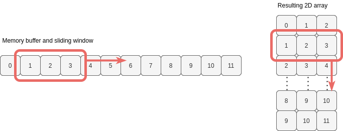
A common use of as_strided is to implement a “sliding window” over an array. For example, a sliding window of size 3 passed over the array a would yield the following 2D array:

We want to end up with an array with shape (10, 3). What strides do we need to specify to achieve this?

For axis 1 (the rows) the jump in memory to the next target integer is 8, as we’re already familiar with. For axis 0 (the jump down a column), notice that we need to jump only 8 bytes again (the values in columns are consecutive). Therefore, the strides we want are (8, 8):

>>> as_strided(a, shape=(10, 3), strides=(8, 8))
array([[ 0,  1,  2],
       [ 1,  2,  3],
       [ 2,  3,  4],
       [ 3,  4,  5],
       [ 4,  5,  6],
       [ 5,  6,  7],
       [ 6,  7,  8],
       [ 7,  8,  9],
       [ 8,  9, 10],
       [ 9, 10, 11]])

So as_strided can be made to make an array look bigger, but with no additional memory required.

A fact not mentioned yet is that strides can be 0 (i.e. don’t jump anywhere), so we can take this one step further and create a large multi-dimensional array from just a single value in memory:

>>> single_value = np.array(0)
>>> as_strided(single_value, (1000, 1000), strides=(0, 0))
array([[0, 0, 0, ..., 0, 0, 0],
       [0, 0, 0, ..., 0, 0, 0],
       [0, 0, 0, ..., 0, 0, 0],
       ...,
       [0, 0, 0, ..., 0, 0, 0],
       [0, 0, 0, ..., 0, 0, 0],
       [0, 0, 0, ..., 0, 0, 0]])

This is a 2D array with 1-million values, which occupy just 8 bytes of memory.

However, as soon as we want to reshape this view or multiply it by a non-scalar value, NumPy will be forced to copy data and we’ll be hit with the full memory usage of our mega-array. A zero stride length can be potential memory-saving device if we simply want to iterate or compare arrays, though.

ndarray

ndarray is the type of a NumPy array. Calling np.array, np.arange or np.zeros (etc.) will create an object of this type, pointing at the correct data buffer and initialised with the appropriate array attributes.

We can also call this method ourselves to create an array, by providing all of the key ingredients of a NumPy array highlighted at the beginning of Part 1:

• memory buffer
• offset into buffer
• shape
• strides

>>> a.reshape(3, 2, 2)[:, ::-1]
array([[[ 2,  3],
        [ 0,  1]],

       [[ 6,  7],
        [ 4,  5]],

       [[10, 11],
        [ 8,  9]]])

>>> np.ndarray(buffer=a.data, shape=(3, 2, 2), strides=(32, -16, 8), offset=16, dtype=int)
array([[[ 2,  3],
        [ 0,  1]],

       [[ 6,  7],
        [ 4,  5]],

       [[10, 11],
        [ 8,  9]]])

As you can see, the ability to specify the offset into the buffer (a.data) allows us even more flexibility than as_strided. We wouldn’t have been able to construct the reverse slice view shown above using as_strided.

But again, why bother to specify strides directly to build views onto a memory buffer?

In my opinion, now we know how NumPy uses strides to traverse memory, it can be easier to solve certain kinds of problems by figuring out what strides to use than by attacking the problems with the higher-level methods such as reshape and transpose.

2. Solving a Stride Problem: Swapping Tiles

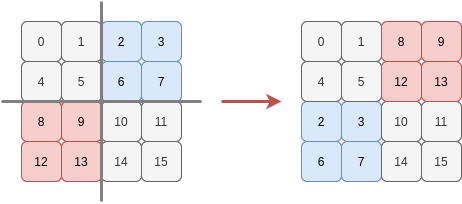
Consider an array with four rows and four columns and imagine it divided into quarters, with each quarter being a two-by-two tile. Suppose we want to swap the top-right tile with the bottom-left tile:

We could slice the array into quarters and then stick them back together in the desired order:

>>> a = np.arange(16).reshape(4, 4)
>>> a
array([[ 0,  1,  2,  3],
       [ 4,  5,  6,  7],
       [ 8,  9, 10, 11],
       [12, 13, 14, 15]])

>>> np.vstack((np.hstack((a[0:2, 0:2], a[2:4, 0:2])), np.hstack((a[0:2, 2:4], a[2:4, 2:4]))))
array([[ 0,  1,  8,  9],
       [ 4,  5, 12, 13],
       [ 2,  3, 10, 11],
       [ 6,  7, 14, 15]])

But that’s too easy. Instead, let’s try and do this by specifying the shape and strides NumPy should use to traverse the values in the order needed to give us our desired “swapped tile” array. What tuple of strides can we use to do this?

We’ll start by looking at the first row. In the original array a, this has a constant stride length to pick out the values [0, 1, 2, 3]:

But in our target array, we want the sequence of values [0, 1, 8, 9]. We need two different stride lengths here!

Two stride lengths means we must have two dimensions, so each of the four rows in our target array needs to be viewed as a sub-array of shape (2, 2) and strides (64, 8). When NumPy traverses each of these 2D subarrays, we’ll get back the values for our rows.

Next, let’s see how to move down columns (i.e. move from one row to the next).

In the original array all we needed was a single stride length to visit the values in the first column [0, 4, 8, 12]:

But now the first column we want is [0, 4, 2, 6]:

Hmmm. Now we have to stride forwards, then seemingly backwards, then forwards again.

How should we handle this backwards stride? Well, the different strides mean we’ll need another two dimensions for sure. It makes most sense to think of the first two rows separately to the second two rows.

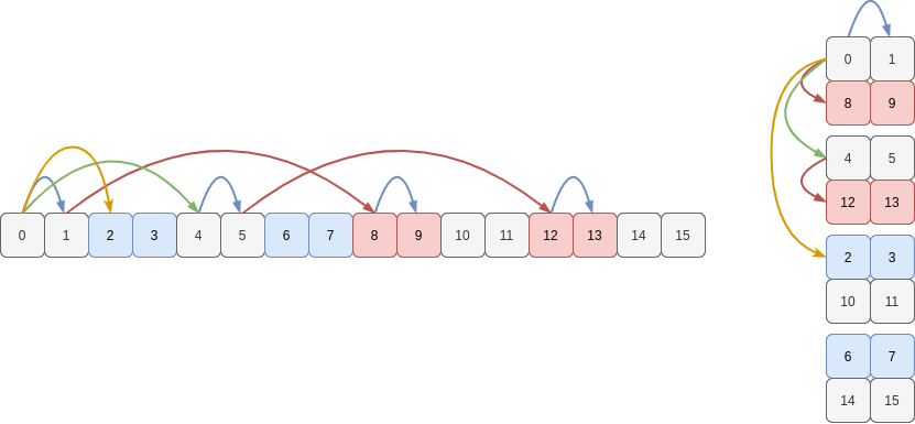
To move down a column from row 0 to row 1, and from row 2 to row 3, both require a stride of 32 bytes. That’s two 3D sub-arrays of shape (2, 2, 2), each with strides (32, 64, 8).

Now, we know that the shape we need is 4D: (2, 2, 2, 2). What is the remaining stride we need to move down a column from the first 3D subarray to the other 3D subarrays? Looking again we only jump 16 bytes. So this initial dimension has a stride of 16 bytes.

Therefore to describe how to visit each value of the memory buffer in the “swapped tile” order, the view onto the memory must have shape (2, 2, 2, 2) and use the strides (16, 32, 64, 8). In the following figure, I’ve sketched some of the strides to navigate the buffer (in C order): blue (8), red (64), green (32) and yellow (16):

If we plug these into as_strided to view a differently we do indeed see the tiles we need, arranged in the order we want them to be to create the rows of our “swapped tile” array:

>>> b = as_strided(a, shape=(2, 2, 2, 2), strides=(16, 32, 64, 8))
>>> b
array([[[[ 0,  1],
         [ 8,  9]],

        [[ 4,  5],
         [12, 13]]],


       [[[ 2,  3],
         [10, 11]],

        [[ 6,  7],
         [14, 15]]]])

We could also have used a combination of reshaping and transposing to create these particular shape and strides, for example a.reshape(2, 2, 2, 2).swapaxes(0, 2). I find it easier to reason using the strides directly, but if you’re good at visualising the results of permuting axes, you might opt for this approach instead.

Anyway, a final reshape back to two dimensions copies the values into a new memory buffer and returns our array:

>>> b.reshape(4, 4)
array([[ 0,  1,  8,  9],
       [ 4,  5, 12, 13],
       [ 2,  3, 10, 11],
       [ 6,  7, 14, 15]])

And there we have the reason why four dimensions are necessary for swapping 2D tiles.