Welcome to the first part of a three-part illustrated guide examining shapes, strides and multidimensionality in NumPy.

The idea of strided arrays is simple, and is a basis for implementing arrays, matrices and tensors in many higher-level languages and frameworks including TensorFlow and Julia.

Strides allow solutions to mind-bending multi-dimensional problems. A better understanding of how they work could make you a more efficient programmer! Practicalities aside, the concept is elegant and worthy of study in its own right.

This post, Part 1, will cover the following topics:

1. Array Fundamentals
2. How Shape and Strides Define Dimensions
3. When Reshaping Copies Data

Part 2 covers:

1. C vs. Fortran order
2. Ravelling
3. Transposing and Permuting Axes

Finally, Part 3 will cover methods to specify the strides of an array directly, and how this can be useful for solving problems:

1. Specifying Strides Directly
2. Stride Study: Swapping Tiles

The intended audience for these posts who have used NumPy already, but have not yet seriously scratched below the surface of how multi-dimensional arrays are implemented.

If you’re already an experienced user of NumPy (or a similar array-based language/library), the chances are you’ll know at least some of the material. However, I hope you’ll still find the presentation of interest.

1. Array Fundamentals

Let’s first establish what a NumPy array is made of.

In a Python shell, create a NumPy array holding 12 integer values:

>>> import numpy as np
>>> a = np.arange(12)
>>> a
array([ 0,  1,  2,  3,  4,  5,  6,  7,  8,  9, 10, 11])

a now identifies a 1-dimensional array object holding 12 integers. It can be sliced, summed and mutated and it appears superficially similar to a familiar Python list object.

Unlike lists, NumPy arrays have not just length, but also shape. In this case a has shape (12,). This single-item tuple means that the array’s single dimension has length 12.

Arrays need not be 1-dimensional though. For example, we can create a 2-dimensional array from a using the reshape method:

>>> b = a.reshape(3, 4)
>>> b
array([[ 0,  1,  2,  3],
       [ 4,  5,  6,  7],
       [ 8,  9, 10, 11]])

Now b is an array with four columns and three rows, holding the same 12 integers. We could easily reshape a to create 3D array, or a 4D array, or any array up to NumPy’s hard limit of 32 dimensions.

The interesting point to make is that to create the 2D array b, NumPy did not duplicate or reorder the integer values used by a. It only had to compute new shape and strides metadata to view these integer values differently.

To put it more plainly: a and b are separate Python objects, but both share the bytes stored in the same bit of memory:

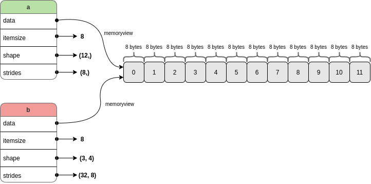
Some key array attributes were highlighted above in the diagram above. In more detail:

• a.data returns a memoryview of the underlying buffer holding the twelve integers.
• a.itemsize is the number of bytes occupied by a single item in the buffer (each item uses the same number of bytes).
• a.shape holds the length of each dimension of the array.
• a.strides holds the number of bytes needed to advance one value along each dimension.

The offset (or “start”) of the buffer is also tracked internally by NumPy (as far as I know it is not exposed as an attribute of the array, see the internal attribute here). This tells NumPy where to begin reading from: not necessarily at the first memory address covered by the buffer.

Now, a fundamental point that I want to get across in this series of posts is this:

Array operations such as reshaping, transposing, indexing, slicing can be thought of as convenient high-level methods to manipulate shape, strides and offset to change how data in memory is traversed.

Two topics which I think are key to understanding how shape and strides work together are indexing and slicing (roughly: getting parts of a larger array), and array iteration (using shape and strides to navigate the memory to return values in a defined sequence).

2. How Shape and Strides Define Dimensions

1-Dimension

a is our 1D array array([ 0, 1, 2, 3, 4, 5, 6, 7, 8, 9, 10, 11]). It has the following shape and strides set by NumPy on construction:

>>> a.shape
(12,)
>>> a.strides
(8,)

The shape (12,) means that the single dimension of a has length 12. There is also a corresponding stride of 8 for this dimension.

The stride indicates the number of bytes to jump in order to reach the next value in the dimension (commonly known as axis) of travel. It is always an integer, and it is always constant for a given axis:

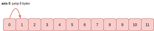
The 8 byte stride matches the itemsize attribute: to read (or jump) one value, this many bytes has to be read (or jumped). For a smaller data type such as int8, then the itemsize would be 1 byte and the stride would also be 1 byte.

Indexing and Slicing

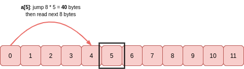
To get a value at a particular index of this array, say a[5], the stride is multiplied by the index value to get the number of bytes to move from the start of the buffer to read itemsize-many bytes:

Just like Python lists, arrays can be sliced. For example, a[::2] returns every other value from the array:

>>> a2 = a[::2]
>>> a2
array([ 0,  2,  4,  6,  8,  10])
>>> a2.shape
(6,)
>>> a2.strides
(16,)

a2 is a new array object which uses the same memory as a, it just interprets it differently using a different shape and strides. a2 reads the memory buffer like this:

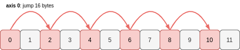
Six values, each separated by a stride of 16 bytes. If the stride if doubled, the length of the axis (the shape) must be halved.

Now let’s see every third value of a, working backwards from the end of the array:

Note that if you reverse an array, the stride changes sign (becomes negative if it was previously positive, and vice-versa). The offset into the memory buffer will also change as NumPy must begin reading from the opposite end.

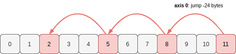
>>> a_reversed = a[::-3]
>>> a_reversed
array([11,  8,  5,  2])
>>> a_reversed.shape
(4,)
>>> a_reversed.strides
(-24,)

The axis of a_reversed has length 4. To get these 4 values, a_reversed begins at the end of the same memory buffer as a and jumps -24 bytes at a time to get to the next item:

These 1D examples demonstrate how the shape and stride attributes of an array determine which values in a region of memory are part of the array, and the order that they take.

Iteration

Iteration over the sequence of values in a 1D array is straightforward.

When NumPy needs to iterate over the values in a (e.g. to sum them with a.sum()), it can see that there are 12 values along the axis (i.e. a.shape[0]), with each one separated by 8 bytes. It knows where to begin reading from in the memory buffer (the offset) and to get the next item it jumps 8 bytes forward to the new memory address.

For slices, the start position in the buffer will change along with the shape (and possibly the stride if a step parameter has been used), but the idea is exactly the same.

N-Dimensions

The same ideas for apply in all higher dimensions. The array just has more axes and NumPy must keep track of how to move between these axes when traversing the items in sequence.

Let’s look again at b, our 2D array with three rows and four columns:

>>> b = a.reshape(3, 4)
>>> b
array([[ 0,  1,  2,  3],
       [ 4,  5,  6,  7],
       [ 8,  9, 10, 11]])

b has two axes, so its shape and stride tuples each have two elements:

>>> b.shape
(3, 4)
>>> b.strides
(32, 8)

To move down one place in a column (axis 0), 32 bytes need to be skipped. To move one place along a row (axis 1), the distance is only 8 bytes:

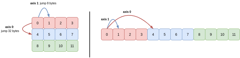
We can see also that the values for each of the three rows are stored together in memory. NumPy defaults to row-major order (“C order”), meaning that elements on rows (higher axes) are closer together in memory than columns (lower axes). We’ll look at the column-major order (Fortran order) in Part 2 of this series.

Indexing and Slicing

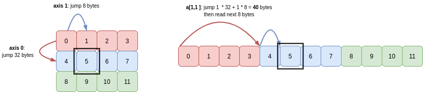
Extending Python’s indexing syntax, NumPy allows you to index/slice each dimension of an array separately.

For example, to get the value in row 1, column 1 of b, you write b[1, 1]. NumPy computes the number of bytes it needs to jump from the start of the buffer in order to retrieve this value:

Through Python’s indexing semantics, we can slice out a view of part of b. For example, let’s get the second and third row, and second and third columns:

>>> b1 = b[1:3, 1:3]
>>> b1
array([[ 5,  6],
       [ 9, 10]])

>>> b1.shape
(2, 2)
>>> b1.strides
(32, 8)

Now b1 is another 2D array with two rows and two columns. Yet again, this a new view onto the same memory buffer as b uses (and therefore the same buffer a uses).

You can see that the shape is (2, 2) and the strides are the same as for b: (32, 8). The other key difference between b1 and b is that the starting point in that memory buffer is different.

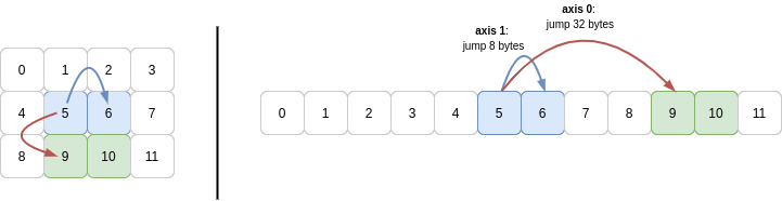
So to slice out this subarray, NumPy begins 40 bytes into the array (same as for b[1, 1]) and reads 8 bytes, then another 8 bytes for the next column in the first row. With that done, to get to the second row, NumPy must jump 32 bytes from the initial 40 offset, so the next row starts 72 bytes into the buffer.

All of these ideas apply in higher dimensions too. Briefly, let’s look a 3D array:

>>> c = a.reshape(3, 2, 2)
>>> c
array([[[ 0,  1],
        [ 2,  3]],

       [[ 4,  5],
        [ 6,  7]],

       [[ 8,  9],
        [10, 11]]])

To navigate the axes of this array, NumPy uses the strides (32, 16, 8):

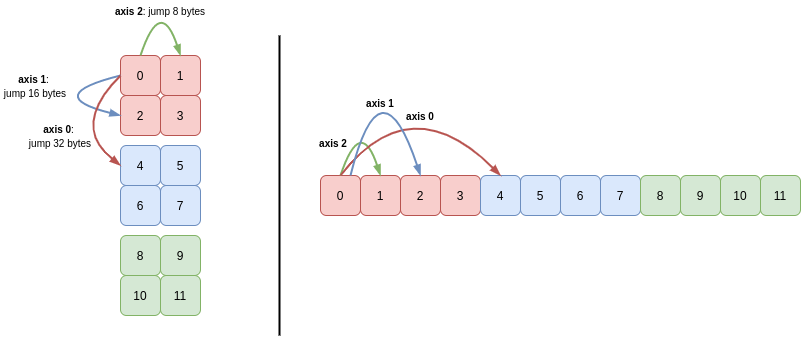
Again, you can see that C order means that NumPy must use a greater stride length to traverse the lower axes than the higher axes.

Iteration

When iterating over arrays with two or more dimensions, NumPy computes and makes use of backstrides for each axis. These values tell NumPy how far it needs to jump back once it reaches the end of each axis, before it can advance along the next axis.

To iterate over all items the 2D array b, the backstride for axis 1 tells NumPy how to get back to the beginning of the row, before it can move down the column (axis 0). The backstride is the length of the axis minus 1, multiplied by the stride for that axis. For axis 1, this is (4 - 1) * 8 == 24:

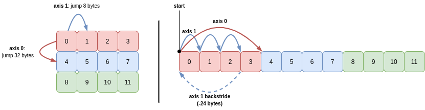
In English, this means the algorithm for visiting all items in the 2D array b in sequence is as follows:

1. Read 8 bytes (b.itemsize) from pointer to get the integer, then move pointer 8 bytes (b.strides[1])
2. Repeat step 2 a total of 3 times (b.shape[1] - 1), then read 8 bytes (read last integer in the row)
3. Move pointer -24 bytes (minus backstride for axis 1)
4. Advance 32 bytes (b.strides[0])
5. Repeat steps 1-4 a total of 3 times to read the remaining rows (b.shape[0])

If we slice out subarrays of the 3D (e.g. c[1:3, :, :1] or c[:, ::-1]), you’ll see that the strides for each axis retain the same magnitude, or are scaled by multiplying by the step, if given (e.g. a step of 2 will multiply the stride for that axis by 2). Other than that, it’s just the shape and the initial offset into the buffer that NumPy needs to adjust.

So for c[:, ::-1] (which just reverses the second axis of c), the strides are (32, -16, 8). To iterate through this array in sequence, the start position is part-way into the memory buffer, at value 2.

The sequence of strides taken to read the first four integers (2, 3, 0, 1) and then move along axis 0 to integer 4 is as follows:

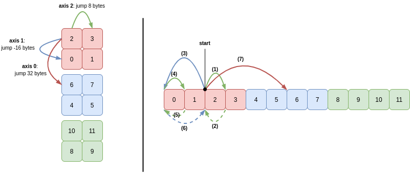
In words:

1. Read 8 bytes (integer 2) and then move 8 bytes (axis 2) to the next memory address
2. Read 8 bytes (integer 3) and then move -8 bytes (backstride for axis 2)
3. Move -16 bytes to advance along axis 1
4. Read 8 bytes (integer 0) and then move 8 bytes (axis 2) to the next memory address
5. Read 8 bytes (integer 1) and then move -8 bytes (backstride for axis 2)
6. Move 16 bytes (backstride for axis 1)
7. Move 32 bytes to advance along axis 1

Steps 1 to 6 then repeat to read the integers 6, 7, 4 and 5.

3. Impossible Reshapes

In each of the examples above, the reshaping, indexing and slicing operations created a new view of the underlying memory by adjusting the shape and strides used to read it. This meant that the same memory buffer could be reused and no copying was necessary.

However, it is not always possible to reshape an array and avoid copying data.

Take the array b1 from above. This was a view of a buffer created from a larger 2D array:

Now let’s try and reshape b1 into a 1D array by setting the .shape attribute directly, which tries to change the shape in C order (traversing higher axes first - more on order in Part 2):

>>> b1.shape = (4,)
Traceback (most recent call last):
  File "<stdin>", line 1, in <module>
AttributeError: incompatible shape for a non-contiguous array

(If we had used b1.reshape(4) the operation would have succeeded because NumPy would have silently copied the values into a new memory buffer.)

The reason this happens is because the stride for an axis has to be constant. Here we need to jump 8 bytes, then 24 bytes, then 8 bytes again to move between the four values in sequence:

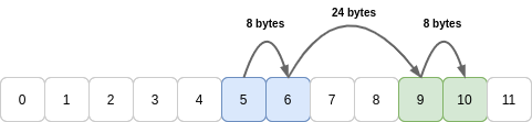
Whenever it cannot hit all values in a row or column using a constant stride length, the reshape method will copy the values into a new buffer. For large arrays this copying can be noticeable: in extreme cases NumPy may even fail to allocate memory!

Summary

In this post, the fundamental attributes used to define NumPy arrays were introduced, and it was demonstrated how array operations such as indexing and reshaping manipulated these attributes to change how data is read from memory.

Part 2 continues this theme and examines how other high-level array operations are expressed as manipulations of these attributes.