Part 2 follows on from the key concepts of strided arrays introduced in the previous post and examines how NumPy implements other fundamental array concepts using strides:

1. Transposing Arrays and Permuting Axes
2. C order vs. Fortran order
3. Ravelling Arrays

1. Transposing Arrays and Permuting Axes

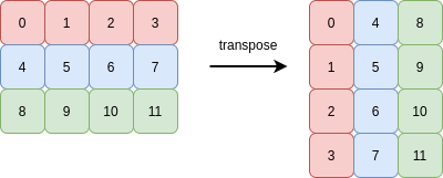
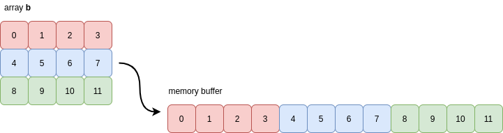
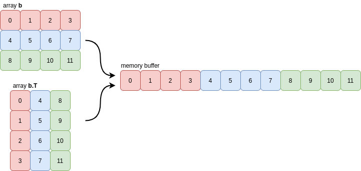
Transposing an array means reversing the order of its axes. The transpose of a 1D array is itself. The simplest interesting case is a 2D array. Rows become columns, and columns become rows:

We saw in part 1 how reshape operations changed an array’s strides to avoid copying data.

When transposing an array, all that NumPy has to do is reverse the array’s shape and the corresponding strides. For example, a shape of (3, 4) becomes (4, 3), and stride tuple is also reversed. This also achieves the goal of the operation without copying data!

The following picture demonstrates this (the memory buffer holding the 12 integers is shown on the right-hand side):

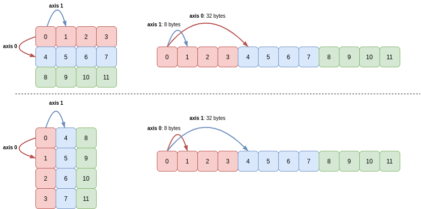
The starting point in the buffer did not need to change, nor did any other array attributes.

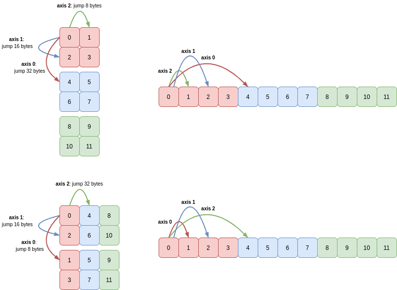
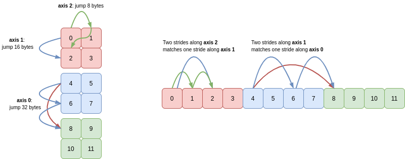
This same principle holds true in higher dimensions too. Consider a 3D array c which has shape (3, 2, 2) and strides (32, 16, 8):

>>> a = np.arange(12)
>>> c = a.reshape(3, 2, 2)
>>> c
array([[[ 0,  1],
        [ 2,  3]],

       [[ 4,  5],
        [ 6,  7]],

       [[ 8,  9],
        [10, 11]]])

Transposing c creates a new array with shape (2, 2, 3) and strides (8, 16, 32):

>>> c.T
array([[[ 0,  4,  8],
        [ 2,  6, 10]],

       [[ 1,  5,  9],
        [ 3,  7, 11]]])

Again, a picture makes this result clearer: axis 0 and axis 2 and their corresponding lengths and strides are swapped:

Even if we permute the axes of a slice of an array no data is copied! For instance if we slice c to take every other entry in axis 0 (cutting out the middle 2x2 array) and then swap axes 0 and 1 we get the following array:

>>> c[::2, :, :].swapaxes(0, 1)
array([[[ 0,  1],
        [ 8,  9]],

       [[ 2,  3],
        [10, 11]]])

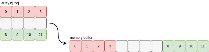
This is still a view of c (and therefore of our 1D array a!) as we’ve just modified how we stride through memory (I’ve greyed-out the region of memory omitted by the slice):

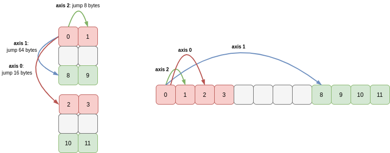
In fact this diagram makes it obvious that we could have permuted the axes 0 and 1 first, then sliced axis 1, since slicing just causes the stride of that axis to increase:

>>> c.swapaxes(0, 1)[:, ::2, :]
array([[[ 0,  1],
        [ 8,  9]],

       [[ 2,  3],
        [10, 11]]])

Thus slicing axes and then swapping them is identical to swapping axes and then slicing them, which perhaps isn’t immediately obvious but is easy enough to see with a diagram.

2. C order vs. Fortran order

This is a good point to nail down the concept of array contiguity.

This topic is implicit in the transpose figures shown above, but let’s see how and why NumPy detects and why it is a useful property of arrays.

First, let’s state what contiguity actually is. We’ll look again at the 2D array b we transposed above:

>>> a = np.arange(12)
>>> b = a.reshape(3, 4)
>>> b
array([[ 0,  1,  2,  3],
       [ 4,  5,  6,  7],
       [ 8,  9, 10, 11]])

If we inspect the array’s .flags attribute, we can see that NumPy has identified it as C contiguous:

>>> b.flags
  C_CONTIGUOUS : True
  F_CONTIGUOUS : False
  ...

This means that NumPy has detected that every row of the array b is grouped together in memory:

For this reason, you may also see the values of C contiguity referred to as being stored in row-major order. NumPy typically defaults to creating arrays as C contiguous when it has to allocate a new memory buffer to hold the array’s contents.

The transpose of the array b is Fortran contiguous (and not C contiguous) meaning that every column of the array is grouped together in memory:

>>> b.T.flags
  C_CONTIGUOUS : False
  F_CONTIGUOUS : True
  ...

NumPy actually uses a very strict notion of contiguity for most of its internal operations: as well as the requirement that values in each row must be grouped together, the rows themselves must also be grouped together (similarly for columns). This means that slices of contiguous arrays are not necessarily contiguous:

>>> b[::2].flags
  C_CONTIGUOUS : False
  F_CONTIGUOUS : False
  ...

Before answering the question of why this matters, let’s look at what NumPy is actually checking and see how the notion of contiguity generalises to higher dimensions.

Unsurprisingly NumPy looks at the array’s strides, together with its shape. Paraphrasing a comment in the NumPy codebase, a contiguous array must satisfy the following two criteria:

1. the leading stride must be the same number of bytes as the array’s itemsize attribute.
2. for all other axes, a single stride along the axis must land you in the same place as taking N many strides of length S, where these letters represent the length and stride of the preceding axis.

For C contiguity, the leading axis is the last axis and NumPy works backwards from there. For F contiguity, axis 0 is the leading axis and NumPy works forwards through the remaining axes. Take c = a.reshape(3, 2, 2) as an example:

So, finally, why does NumPy bother to perform this contiguity check? Performance.

Firstly performance is important when NumPy needs to visit the items of this array in sequence, for example to sum them up.

As we saw in the previous post, this ordering is defined by the array’s shape and strides. NumPy will hop around memory as these strides dictate to visit the items in the array. There’s a fantastic bit of machinery, the Multidimensional Iterator, for handling this hopping around the buffer. For contiguous arrays though, where every hop is just to the adjacent memory address, the overhead of this iterator is not needed and NumPy can blaze straight through the buffer (possibly employing CPU-specific optimisations).

Secondly, there are performance considerations for reshaping strategies too. If NumPy knows the contents of the array are in a neat order and the user wants to visit the contents in that same neat order, NumPy can return a view onto the array rather than copying data.

To expand on this second point, the considerations in array order and contiguity are especially obvious when ravelling arrays.

Ravelling

Ravelling a multidimensional array means placing all of its values onto a single axes, in a given order.

NumPy will walk the axes of the array in this order, picking up the values of the array. For C order or F order, this is a special case of reshaping, equivalent to array.reshape(-1, order=order). As with reshaping, ravelling an array will create a view instead of leading to copying values from the underlying buffer if the array is contiguous.

For C order, the axes are traversed from high to low (axis 0). The one dimensional array at the top is the result of ravelling the other C-contiguous arrays in C order. There’s an obvious “Z” pattern in the way the rows and columns are traversed in higher dimensions:

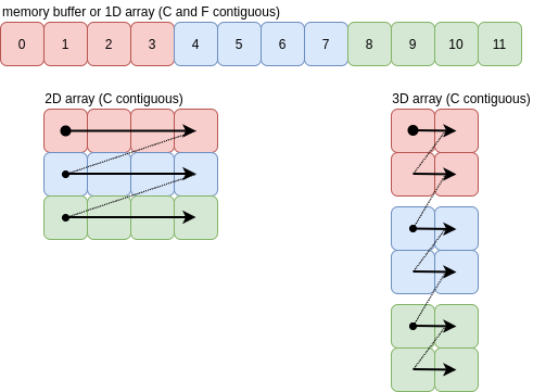
The “Z” pattern continues beyond three dimensions, which is easy to visualise. In all cases the arrows represent a single jump of itemsize bytes.

For this case, where each arrow leads to the value adjacent in the memory buffer, the array is contiguous and ravelling can be done with a new view onto the existing memory buffer.

For F order, the axes of the array are traversed from low to high. The images below show F contiguous arrays and the order the values are pushed onto a single axis. Once you get to three dimensions the picture looks more complicated than C order, but the idea is exactly the same:

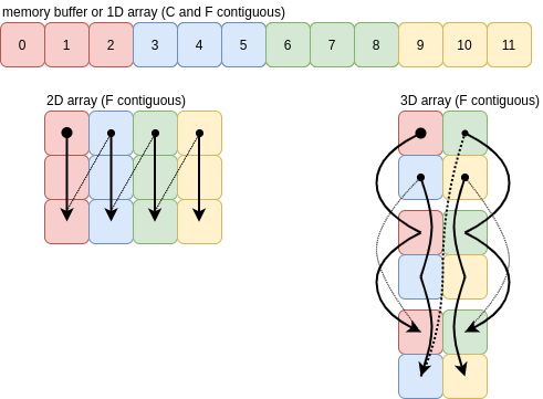
As long as the array is F contiguous, ravelling in F order will just create a new view of the buffer.

As Part 1 of this series closed with an “impossible to view” reshape, let’s close Part 2 with such a ravel.

If we take a C contiguous array and try to ravel it in F order, NumPy has to jump forwards and backwards in the memory buffer as it follows the strides for each axis in ascending order:

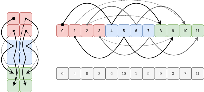
There’s simply no way to visit the elements of the existing buffer in this order using a constant stride, so NumPy copies them into a new buffer in this oscillating sequence to use for the ravelled array.