If you’ve played about with NumPy before, you’ll probably know that given two arrays of numbers, ar1 and ar2, the function in1d returns a boolean array indicating whether or not each number in ar1 appears somewhere in ar2. Very useful!

To compute this boolean array, one of two paths is taken inside np.in1d. The default path involves finding the unique values in the two arrays, then combining, sorting and comparing them. However, if ar2 is somewhat shorter than ar2, a faster code path can be taken to avoid the overhead of sorting.

Specifically, to see if ar2 is short enough relative to ar1, the following inequality is used:

if len(ar2) < 10 * len(ar1) ** 0.145:
    # iterate over ar2 and compare it to each element in ar1

For instance if ar1 had length 1000, the faster path would be taken only if ar2 had 27 or fewer elements. Very interesting! Where does this magic number 0.145 come from?

Initially I thought that the constants in the inequality could be approximated analytically. I started adding up the complexity of the sorting and indexing routines used in the default path, scribbled some vague equations, and got absolutely nowhere. Then I had the more sensible thought that the constants were probably derived by running tests and that this might be documented somewhere online. Cue rummaging around GitHub.

It turns out that the fast path with the inequality above was introduced back in 2011 in this commit, crediting the work to Neil Crighton who built on an idea from Robert Kern. It points back to this ticket, which has attachments explaining how the constants were chosen:

I’ve attached a script that compares timings for the existing version of in1d and the kern_in function described in the thread above; I use this to work out which algorithm is fastest for given lengths of ar1 and ar2 (see also the attached plot).

Perfect: the constants were derived by experiment and, whatsmore, the original script to compare the two paths still exists. The following contour plot originally produced by the script was attached (“kern” is the fast path). The key part is the red dotted line which plots the equation 10 * len(ar1) ** 0.145:

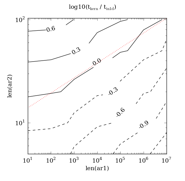
Here the contours are time ratios; the 0.0 contour follows where the fast path and default path were equal. Lower contours show where the fast path is fater, higher contours show where it is slower. We can see that the constants 10 and 0.145 were good choices since the red dotted line nicely approximates the 0.0 contour.

Is it still the case that 0.145 is the best choice today?

NumPy has been developed and improved since 2011, and key indexing and sorting routines have been optimised further. Curious, I re-ran the script on my own machine with only some minor syntactical changes (hello from Python 3). The original red dotted line using the original magic numbers is drawn on for comparison:

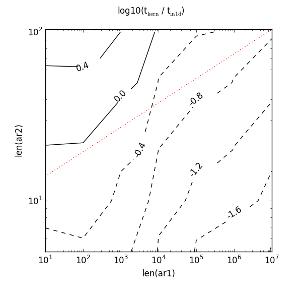
Not so good! Now that red dotted line misses the 0.0 contour completely. It needs a higher value to intercept it and could also do with a steeper gradient. If I were tasked with the tricky problem of picking new constants, it seems reasonable to go with the inequality 8 * len(ar1) ** 0.25. Here’s what that red dotted line looks like:

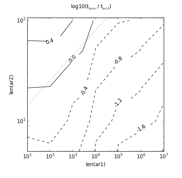
So on my machine, it looks like 8 and 0.25 are better magic numbers than 10 and 0.145.

Interesting graphs aside, I don’t recommend that you rush to patch your in1d function with new “better” constants. If performance really matters, it would better to test which path is faster for the size of arrays you’re working with and then use a custom function containing the speedier code.